life_demo

Example of initialization and fitting of the LiFE model
Build the file names for the diffusion data, the anatomical MRI.
(1) Evaluate the Probabilistic CSD-based connectome.
(1.1) Initialize the LiFE model structure, 'fe' in the code below.
(1.2) Fit the model.
(1.3) Extract the RMSE of the model on the fitted data set.
(1.4) Extract the RMSE of the model on the second data set.
(1.5) Extract the Rrmse.
(1.6) Extract the fitted weights for the fascicles.
(1.7) Plot a histogram of the RMSE.
(1.8) Plot a histogram of the RMSE ratio.
(1.9) Plot a histogram of the fitted fascicle weights.
Extract the coordinates of the white-matter voxels
(2) Evaluate the Deterministic tensor-based connectome.
(2.1) Initialize the LiFE model structure, 'fe' in the code below.
(2.2) Fit the model.
(2.3) Extract the RMSE of the model on the fitted data set.
(2.4) Extract the RMSE of the model on the second data set.
(2.5) Extract the Rrmse.
(2.6) Extract the fitted weights for the fascicles.
(2.7) Plot a histogram of the RMSE.
(2.8) Plot a histogram of the RMSE ratio.
(2.9) Plot a histogram of the fitted fascicle weights.
Extract the coordinates of the white-matter voxels.
(3) Compare the quality of fit of Probabilistic and Deterministic connectomes.
(3.1) Find the common coordinates between the two connectomes.
(3.2) Make a scatter plot of the RMSE of the two tractography models
(3.3) Compute the strength-of-evidence (S) and the Earth Movers Distance.
(3.4) Strength of evidence in favor of Probabilistic tractography.
(3.5) RMSE distributions for Probabilistic and Deterministic tractography.

function [fh, fe] = life_demo()

Example of initialization and fitting of the LiFE model

This demo function illustrates how to: - A - Set up a LiFE structure, identified as 'fe' (fascicle evaluation) in the code below. This model contains a prediction of the diffusion measurements in each white-matter voxel given by the fascicles contained in a tractogrpahy solution, the connectome. Each fascicles makes a prediction about the direction of diffusion in the set of voxels where it travels through. The prediction is generated given the fascicle orientation and position isndie the voxel. Predictions from multiple fascicles in in each voxels are combined to generate a global connectome prediciton for the diffusion signal in large sets of white matter voxels. - B - Fit the LiFE model to compute the weights associated to each fascicle in the connectome. Fascicles in the conenctome contribute differently to predicting the diffusion signal in each voxel. First of all, fascicles make predictions about the diffusion only in voxels where they travel. Secondly, some fascicles have paths that produce better diffusion predictions than others. We use a least-square method to find the contribution of each fascicle to the diffusion signal in the white matter voxels where the fascicles travels. A single weight is assigned to each fascicle representing the global contribution of the fasicle to the signal of all the voxels along its path - we call this fascicle-global. Because multiple fascicles exist in several voxels the set of fascicles weights and fascicles predicitons represents the connectome-global prediction of the diffusion signal within the entire set of white matter voxels. Estimating the fascicle weights allows for evaluating the quality of the tractography solution. Eliminating fascicles that do not contribute to predicting the diffusion signal (they have assigned a zreo-weight). Finaly, the root-mean-squared error (RMSE) of the model to the diffusion data - the model prediction error - is used to evaluate the model prediction quality, compare different tractography models and to perform statistical inference on the on properties of the connectomes. - C - Compare two different connectome models. This demo will show how to compare two different conenctome models by using the diffusion prediction error (the Root-Mean-Squared Error, RMSE). We report the example of two conenctomes one generated using Constrained-spherical deconvolution (CSD) and probabilistic tractography the other using a tensor model and deterministic tractography - D - Not Implemented : Performs a virtual lesion. - Note - The example connectomes used for this demo comprise a portion of the right occiptial lobe of an individual human brain. LiFE utilizes large-scale methods to solve the foward model. The software allows for solving connectomes spanning the entire white-matter of idnvidual brains. The size of the connectome on the test data set is small enought to allow for testing the code within a few minutes requiring only about 10GB of computer RAM and standard hardaware. This code has been tested with: - Ubuntu 12.04.4 LTS (Precise) - 2.6Ghz i7 Processor and 24GB of RAM. - MatLab Version: 8.0.0.783 (R2012b)

% Intialize a local matlab cluster if the parallel toolbox is available.
% This helps speeding up computations espacially for large conenctomes.
feOpenLocalCluster;

[feOpenLocalCluster] Found Matlab parallel cluster open, not intializing.

Build the file names for the diffusion data, the anatomical MRI.

dwiFile       = fullfile(lifeDemoDataPath('diffusion'),'pestilli_etal_life_demo_scan1_subject1_b2000_150dirs_stanford.nii.gz');
dwiFileRepeat = fullfile(lifeDemoDataPath('diffusion'),'pestilli_etal_life_demo_scan2_subject1_b2000_150dirs_stanford.nii.gz');
t1File        = fullfile(lifeDemoDataPath('anatomy'),  'pestilli_etal_life_demo_anatomy_t1w_stanford.nii.gz');

(1) Evaluate the Probabilistic CSD-based connectome.

We will analyze first the CSD-based probabilistic tractography connectome.

prob.tractography = 'Probabilistic';
fgFileName    = fullfile(lifeDemoDataPath('tractography'), ...
                'pestilli_et_al_life_demo_mrtrix_csd_lmax10_probabilistic.mat');

% The final connectome and data astructure will be saved with this name:
feFileName    = 'life_build_model_demo_CSD_PROB';

(1.1) Initialize the LiFE model structure, 'fe' in the code below.

This structure contains the forward model of diffusion based on the tractography solution. It also contains all the information necessary to compute model accuracry, and perform statistical tests. You can type help('feBuildModel') in the MatLab prompt for more information.

fe = feConnectomeInit(dwiFile,fgFileName,feFileName,[],dwiFileRepeat,t1File);

[feOpenLocalCluster] Found Matlab parallel cluster open, not intializing.

[feConnectomeInit]
 loading fiber from file: /marcovaldo/frk/git/life/Pestilli_etal_manuscript/data/tractography/pestilli_et_al_life_demo_mrtrix_csd_lmax10_probabilistic.mat

[feConnectomeInit] Computing fibers' tensors... [feOpenLocalCluster] Found Matlab parallel cluster open, not intializing.
Elapsed time is 3.299457 seconds.
[fefgGet] Computing fibers/nodes pairing in each voxel..
[fefgGet] Computing nodes-to-voxels..[feOpenLocalCluster] Found Matlab parallel cluster open, not intializing.
 took: 0.489minutes.
[fefgGet] Computing voxels-in-fg..[feOpenLocalCluster] Found Matlab parallel cluster open, not intializing.
 took: 0.504s.
[fefgGet] Computing nodes-in-voxels..[feOpenLocalCluster] Found Matlab parallel cluster open, not intializing.
 took: 0.225s.
[fefgGet] fiber/node pairing completed in: 14.925s.

Files loaded: 
  dwi   = /marcovaldo/frk/git/life/Pestilli_etal_manuscript/data/diffusion/pestilli_etal_life_demo_scan1_subject1_b2000_150dirs_stanford.nii.gz 
  bvecs = /marcovaldo/frk/git/life/Pestilli_etal_manuscript/data/diffusion/pestilli_etal_life_demo_scan1_subject1_b2000_150dirs_stanford.bvecs 
  bvals = /marcovaldo/frk/git/life/Pestilli_etal_manuscript/data/diffusion/pestilli_etal_life_demo_scan1_subject1_b2000_150dirs_stanford.bvals


Files loaded: 
  dwi   = /marcovaldo/frk/git/life/Pestilli_etal_manuscript/data/diffusion/pestilli_etal_life_demo_scan2_subject1_b2000_150dirs_stanford.nii.gz 
  bvecs = /marcovaldo/frk/git/life/Pestilli_etal_manuscript/data/diffusion/pestilli_etal_life_demo_scan2_subject1_b2000_150dirs_stanford.bvecs 
  bvals = /marcovaldo/frk/git/life/Pestilli_etal_manuscript/data/diffusion/pestilli_etal_life_demo_scan2_subject1_b2000_150dirs_stanford.bvals

LiFE - Building the connectome model...
LiFE - Predicting diffusion signal in 10694 voxel...
[feOpenLocalCluster] Found Matlab parallel cluster open, not intializing.
LiFE - Prediction computed in: 22.473s.
LiFE - Allocating the model prediction...process completed in 327.057s.
LiFE - DONE Building the connectome model.

(1.2) Fit the model.

Hereafter we fit the forward model of tracrography using a least-squared method. The information generated by fitting the model (fiber weights etc) is then installed in the LiFE structure.

fe = feSet(fe,'fit',feFitModel(feGet(fe,'mfiber'),feGet(fe,'dsigdemeaned'),'bbnnls'));

LiFE: Computing least-square minimization with BBNNLS...
Running: **** SBB-NNLS ****

Iter   	     Obj		  ||pg||_inf		 ||x-x*||
-------------------------------------------------------
0001	 1.307919E+09	6.466619E+07	NaN
0002	 1.243174E+09	3.585529E+07	NaN
0003	 1.208840E+09	2.977730E+07	NaN
0004	 1.159646E+09	2.635689E+07	NaN
0005	 1.147525E+09	2.559348E+07	NaN
0006	 1.136161E+09	1.922265E+07	NaN
0007	 1.130214E+09	1.730660E+07	NaN
0008	 1.110027E+09	1.680250E+07	NaN
0009	 1.089190E+09	1.459978E+07	NaN
0010	 1.078166E+09	1.276464E+07	NaN
0011	 1.038559E+09	5.794384E+07	NaN
0012	 1.034712E+09	2.208430E+07	NaN
0013	 1.033524E+09	9.050799E+06	NaN
0014	 1.026760E+09	8.631986E+06	NaN
0015	 1.022509E+09	2.021612E+07	NaN
0016	 1.021654E+09	8.199957E+06	NaN
0017	 1.021025E+09	8.145108E+06	NaN
0018	 1.014731E+09	8.096567E+06	NaN
0019	 1.001784E+09	3.661682E+07	NaN
0020	 1.000342E+09	1.494266E+07	NaN
0021	 9.998125E+08	7.208974E+06	NaN
0022	 9.980974E+08	5.713491E+06	NaN
0023	 9.951437E+08	2.003736E+07	NaN
0024	 9.947451E+08	7.085062E+06	NaN
0025	 9.944719E+08	5.389950E+06	NaN
0026	 9.924290E+08	5.367824E+06	NaN
0027	 9.861289E+08	3.046906E+07	NaN
0028	 9.856522E+08	5.297671E+06	NaN
0029	 9.852687E+08	4.530251E+06	NaN
0030	 9.833146E+08	4.267369E+06	NaN
0031	 9.824782E+08	5.532911E+06	NaN
0032	 9.820785E+08	4.150418E+06	NaN
0033	 9.818460E+08	4.125086E+06	NaN
0034	 9.751396E+08	4.110650E+06	NaN
0035	 9.738408E+08	9.077890E+06	NaN
0036	 9.733680E+08	1.010801E+07	NaN
0037	 9.732383E+08	5.176729E+06	NaN
0038	 9.762260E+08	3.365940E+06	NaN
0039	 9.716284E+08	2.547585E+07	NaN
0040	 9.712928E+08	3.882891E+06	NaN
0041	 9.710759E+08	3.203070E+06	NaN
0042	 9.688401E+08	3.183377E+06	NaN
0043	 9.685904E+08	3.286071E+06	NaN
0044	 9.681592E+08	2.890947E+06	NaN
0045	 9.678729E+08	2.845161E+06	NaN
0046	 9.621745E+08	2.811581E+06	NaN
0047	 9.619519E+08	6.238817E+06	NaN
0048	 9.616957E+08	4.309485E+06	NaN
0049	 9.614659E+08	3.305908E+06	NaN
0050	 9.610926E+08	2.187766E+06	NaN
0051	 9.609719E+08	2.247655E+06	NaN
0052	 9.608367E+08	1.570873E+06	NaN
0053	 9.607682E+08	2.947223E+06	NaN
0054	 9.606375E+08	1.546544E+06	NaN
0055	 9.604227E+08	1.528272E+06	NaN
0056	 9.599080E+08	1.494245E+06	NaN
0057	 9.587330E+08	1.646919E+07	NaN
0058	 9.585722E+08	5.737623E+06	NaN
0059	 9.584041E+08	4.269265E+06	NaN
0060	 9.581604E+08	3.585277E+06	NaN
0061	 9.581161E+08	2.719826E+06	NaN
0062	 9.580108E+08	1.869510E+06	NaN
0063	 9.578532E+08	6.050375E+06	NaN
0064	 9.578310E+08	1.017997E+06	NaN
0065	 9.577823E+08	1.000609E+06	NaN
0066	 9.581825E+08	9.954103E+05	NaN
0067	 9.569259E+08	1.297705E+07	NaN
0068	 9.568947E+08	1.442907E+06	NaN
0069	 9.568679E+08	8.345098E+05	NaN
0070	 9.566514E+08	8.319305E+05	NaN
0071	 9.565919E+08	1.337015E+06	NaN
0072	 9.565595E+08	1.573419E+06	NaN
0073	 9.565445E+08	1.751876E+06	NaN
0074	 9.565027E+08	7.864680E+05	NaN
0075	 9.564852E+08	7.736305E+05	NaN
0076	 9.563229E+08	7.693740E+05	NaN
0077	 9.562957E+08	9.822361E+05	NaN
0078	 9.562757E+08	7.192193E+05	NaN
0079	 9.562642E+08	7.456113E+05	NaN
0080	 9.561133E+08	7.132708E+05	NaN
0081	 9.559795E+08	6.868294E+05	NaN
0082	 9.559649E+08	1.640678E+06	NaN
0083	 9.559481E+08	2.281374E+06	NaN
0084	 9.559365E+08	6.602509E+05	NaN
0085	 9.559111E+08	6.584714E+05	NaN
0086	 9.555176E+08	6.541630E+05	NaN
0087	 9.554840E+08	2.813916E+06	NaN
0088	 9.554702E+08	1.397569E+06	NaN
0089	 9.554617E+08	8.706310E+05	NaN
0090	 9.554427E+08	7.468709E+05	NaN
0091	 9.554346E+08	1.080044E+06	NaN
0092	 9.554243E+08	5.554830E+05	NaN
0093	 9.554168E+08	5.540269E+05	NaN
0094	 9.552601E+08	5.528034E+05	NaN
0095	 9.551597E+08	7.162165E+06	NaN
0096	 9.550484E+08	5.574252E+06	NaN
0097	 9.550170E+08	2.698502E+06	NaN
0098	 9.549932E+08	2.046093E+06	NaN
0099	 9.549425E+08	3.935970E+06	NaN
0100	 9.549352E+08	9.693352E+05	NaN
0101	 9.549180E+08	7.555799E+05	NaN
0102	 9.549135E+08	1.131412E+06	NaN
0103	 9.549051E+08	1.308309E+06	NaN
0104	 9.549017E+08	8.723968E+05	NaN
0105	 9.548994E+08	5.034316E+05	NaN
0106	 9.548812E+08	3.670025E+05	NaN
0107	 9.548766E+08	6.998372E+05	NaN
0108	 9.548740E+08	3.512696E+05	NaN
0109	 9.548724E+08	3.506403E+05	NaN
0110	 9.548449E+08	3.501907E+05	NaN
0111	 9.548367E+08	3.418272E+05	NaN
0112	 9.548405E+08	6.308415E+05	NaN
0113	 9.548295E+08	1.528593E+06	NaN
0114	 9.548282E+08	3.407951E+05	NaN
0115	 9.548269E+08	3.406979E+05	NaN
0116	 9.546963E+08	3.405933E+05	NaN
0117	 9.546906E+08	1.418370E+06	NaN
0118	 9.546746E+08	1.921842E+06	NaN
0119	 9.546708E+08	1.445751E+06	NaN
0120	 9.547583E+08	6.442646E+05	NaN
0121	 9.546586E+08	4.075085E+06	NaN
0122	 9.546569E+08	3.575407E+05	NaN
0123	 9.546562E+08	2.916773E+05	NaN
0124	 9.546525E+08	2.905436E+05	NaN
0125	 9.546511E+08	2.818912E+05	NaN
0126	 9.546499E+08	2.790210E+05	NaN
0127	 9.546490E+08	2.753583E+05	NaN
0128	 9.546482E+08	2.741964E+05	NaN
0129	 9.546479E+08	2.724172E+05	NaN
0130	 9.546457E+08	2.715859E+05	NaN
0131	 9.546454E+08	2.661786E+05	NaN
0132	 9.546447E+08	2.654132E+05	NaN
0133	 9.546445E+08	2.638853E+05	NaN
0134	 9.546436E+08	2.633569E+05	NaN
0135	 9.546390E+08	2.612590E+05	NaN
0136	 9.566035E+08	2.499422E+05	NaN
0137	 9.554660E+08	1.510042E+07	NaN
0138	 9.553037E+08	5.826542E+06	NaN
0139	 9.550878E+08	4.615684E+06	NaN
0140	 9.549339E+08	3.412313E+06	NaN
0141	 9.548659E+08	3.090428E+06	NaN
0142	 9.548177E+08	3.372325E+06	NaN
0143	 9.547826E+08	2.944437E+06	NaN
0144	 9.547587E+08	1.505082E+06	NaN
0145	 9.547366E+08	1.367243E+06	NaN
0146	 9.548708E+08	1.223587E+06	NaN
0147	 9.546440E+08	6.046396E+06	NaN
0148	 9.546373E+08	1.251820E+06	NaN
0149	 9.546333E+08	6.899156E+05	NaN
0150	 9.546272E+08	5.133182E+05	NaN
0151	 9.546256E+08	5.210804E+05	NaN
0152	 9.546251E+08	3.136826E+05	NaN
0153	 9.546201E+08	1.137994E+06	NaN
0154	 9.546197E+08	1.963965E+05	NaN
0155	 9.546194E+08	2.275986E+05	NaN
0156	 9.546173E+08	2.128939E+05	NaN
0157	 9.546155E+08	5.672008E+05	NaN
0158	 9.546151E+08	2.648349E+05	NaN
0159	 9.546150E+08	1.526309E+05	NaN
0160	 9.546143E+08	1.526752E+05	NaN
0161	 9.546140E+08	1.530146E+05	NaN
0162	 9.546140E+08	1.530923E+05	NaN
0163	 9.546135E+08	2.704254E+05	NaN
0164	 9.546134E+08	1.532447E+05	NaN
0165	 9.546133E+08	1.532524E+05	NaN
0166	 9.546115E+08	1.532604E+05	NaN
0167	 9.546113E+08	1.534815E+05	NaN
0168	 9.546111E+08	1.534050E+05	NaN
0169	 9.546110E+08	1.796172E+05	NaN
0170	 9.546110E+08	1.533040E+05	NaN
0171	 9.546107E+08	1.532572E+05	NaN
0172	 9.546050E+08	1.530805E+05	NaN
0173	 9.546079E+08	6.410887E+05	NaN
0174	 9.546024E+08	9.074573E+05	NaN
0175	 9.546016E+08	7.178098E+05	NaN
0176	 9.546017E+08	3.418290E+05	NaN
0177	 9.546008E+08	4.553512E+05	NaN
0178	 9.546008E+08	1.392320E+05	NaN
0179	 9.546007E+08	1.391771E+05	NaN
0180	 9.546001E+08	1.390597E+05	NaN
0181	 9.546007E+08	1.374120E+05	NaN
0182	 9.546001E+08	3.135992E+05	NaN
0183	 9.545998E+08	3.636200E+05	NaN
0184	 9.545998E+08	1.363430E+05	NaN
0185	 9.545997E+08	1.361783E+05	NaN
0186	 9.545997E+08	1.356925E+05	NaN
0187	 9.545995E+08	1.716984E+05	NaN
0188	 9.545994E+08	1.371773E+05	NaN
0189	 9.545994E+08	4.871785E+04	NaN
0190	 9.545993E+08	4.851467E+04	NaN
0191	 9.545993E+08	4.627005E+04	NaN
0192	 9.545993E+08	4.522115E+04	NaN
0193	 9.545993E+08	7.553992E+04	NaN
0194	 9.545993E+08	4.422537E+04	NaN
0195	 9.545993E+08	4.396856E+04	NaN
0196	 9.545987E+08	4.360215E+04	NaN
0197	 9.546010E+08	3.736175E+04	NaN
0198	 9.546039E+08	5.593638E+05	NaN
0199	 9.545987E+08	1.258238E+06	NaN
0200	 9.545986E+08	1.503108E+05	NaN
0201	 9.545986E+08	9.476199E+04	NaN
0202	 9.545986E+08	7.737394E+04	NaN
0203	 9.545985E+08	2.460752E+04	NaN
0204	 9.545985E+08	2.197667E+04	NaN
0205	 9.545985E+08	3.865351E+04	NaN
0206	 9.545985E+08	2.053351E+04	NaN
0207	 9.545985E+08	2.056268E+04	NaN
0208	 9.545985E+08	2.057528E+04	NaN
0209	 9.545985E+08	2.063163E+04	NaN
0210	 9.545994E+08	2.020928E+04	NaN
0211	 9.545984E+08	3.810580E+05	NaN
0212	 9.545984E+08	4.631575E+04	NaN
0213	 9.545984E+08	2.125731E+04	NaN
0214	 9.545984E+08	1.894896E+04	NaN
0215	 9.545984E+08	1.866600E+04	NaN
0216	 9.545983E+08	1.851019E+04	NaN
0217	 9.545983E+08	1.802152E+04	NaN
0218	 9.545983E+08	1.751355E+04	NaN
0219	 9.545983E+08	1.751099E+04	NaN
0220	 9.545983E+08	1.750111E+04	NaN
0221	 9.545983E+08	1.742603E+04	NaN
0222	 9.546020E+08	1.717089E+04	NaN
0223	 9.546018E+08	7.398353E+05	NaN
0224	 9.545985E+08	6.621276E+05	NaN
0225	 9.545982E+08	5.163443E+05	NaN
0226	 9.545981E+08	2.189606E+05	NaN
0227	 9.545980E+08	1.723451E+05	NaN
0228	 9.545980E+08	7.894258E+04	NaN
0229	 9.545980E+08	7.782025E+04	NaN
0230	 9.545980E+08	4.827688E+04	NaN
0231	 9.545980E+08	1.581160E+04	NaN
0232	 9.545980E+08	7.452975E+03	NaN
0233	 9.545980E+08	7.449612E+03	NaN
0234	 9.545980E+08	7.446599E+03	NaN
0235	 9.545980E+08	7.428032E+03	NaN
0236	 9.545980E+08	7.414423E+03	NaN
0237	 9.545980E+08	2.374671E+04	NaN
0238	 9.545980E+08	7.371639E+03	NaN
0239	 9.545980E+08	7.365412E+03	NaN
0240	 9.545979E+08	7.355580E+03	NaN
0241	 9.545981E+08	3.618382E+04	NaN
0242	 9.545981E+08	1.902163E+05	NaN
0243	 9.545979E+08	2.015312E+05	NaN
0244	 9.545979E+08	2.993021E+04	NaN
0245	 9.545979E+08	2.022173E+04	NaN
0246	 9.545979E+08	1.916649E+04	NaN
0247	 9.545979E+08	8.887401E+03	NaN
0248	 9.545979E+08	4.638121E+03	NaN
0249	 9.545979E+08	8.301623E+03	NaN
0250	 9.545979E+08	3.705061E+03	NaN
0251	 9.545979E+08	3.682267E+03	NaN
0252	 9.545979E+08	3.654972E+03	NaN
0253	 9.545980E+08	4.729992E+03	NaN
0254	 9.545982E+08	6.268547E+04	NaN
0255	 9.545979E+08	1.998843E+05	NaN
0256	 9.545979E+08	9.482112E+03	NaN
0257	 9.545979E+08	4.202085E+03	NaN
0258	 9.545979E+08	3.338180E+03	NaN
0259	 9.545979E+08	3.336885E+03	NaN
0260	 9.545979E+08	3.334053E+03	NaN
0261	 9.545979E+08	3.504531E+03	NaN
0262	 9.545979E+08	6.319085E+03	NaN
0263	 9.545979E+08	6.998167E+03	NaN
0264	 9.545979E+08	3.193358E+03	NaN
0265	 9.545979E+08	3.189586E+03	NaN
0266	 9.545979E+08	3.186388E+03	NaN
0267	 9.545979E+08	3.094940E+03	NaN
0268	 9.545979E+08	5.187398E+03	NaN
0269	 9.545979E+08	8.946178E+03	NaN
0270	 9.545979E+08	3.082129E+03	NaN
0271	 9.545979E+08	3.080241E+03	NaN
0272	 9.545979E+08	3.077652E+03	NaN
0273	 9.545979E+08	2.977499E+03	NaN
0274	 9.545979E+08	2.965755E+03	NaN
0275	 9.545979E+08	2.960223E+03	NaN
0276	 9.545979E+08	2.956179E+03	NaN
0277	 9.545979E+08	2.951984E+03	NaN
0278	 9.545979E+08	2.949720E+03	NaN
0279	 9.545979E+08	2.941600E+03	NaN
0280	 9.545981E+08	2.910159E+03	NaN
0281	 9.545979E+08	1.750778E+05	NaN
0282	 9.545979E+08	1.995156E+04	NaN
0283	 9.545979E+08	2.244861E+03	NaN
0284	 9.545979E+08	1.926622E+03	NaN
0285	 9.545979E+08	1.924279E+03	NaN
0286	 9.545979E+08	1.922280E+03	NaN
0287	 9.545979E+08	1.913543E+03	NaN
0288	 9.545979E+08	1.910503E+03	NaN
0289	 9.545979E+08	1.908445E+03	NaN
0290	 9.545979E+08	1.906896E+03	NaN
0291	 9.545979E+08	1.902678E+03	NaN
0292	 9.545979E+08	1.901029E+03	NaN
0293	 9.545979E+08	1.866193E+03	NaN
0294	 9.545979E+08	1.864115E+03	NaN
0295	 9.545979E+08	1.862195E+03	NaN
0296	 9.545979E+08	1.860880E+03	NaN
0297	 9.545979E+08	1.849046E+03	NaN
0298	 9.545982E+08	1.785784E+03	NaN
0299	 9.545980E+08	1.785988E+05	NaN
0300	 9.545979E+08	1.356141E+05	NaN
0301	 9.545979E+08	8.559631E+04	NaN
0302	 9.545979E+08	4.391639E+04	NaN
0303	 9.545979E+08	1.517606E+04	NaN
0304	 9.545979E+08	3.277346E+03	NaN
0305	 9.545979E+08	1.697454E+03	NaN
0306	 9.545979E+08	1.192846E+03	NaN
0307	 9.545979E+08	1.399884E+03	NaN
0308	 9.545979E+08	8.133494E+02	NaN
0309	 9.545979E+08	1.757236E+03	NaN
0310	 9.545979E+08	7.237174E+02	NaN
0311	 9.545979E+08	1.079226E+03	NaN
0312	 9.545979E+08	8.863143E+02	NaN
0313	 9.545979E+08	8.687135E+02	NaN
0314	 9.545979E+08	7.706611E+02	NaN
0315	 9.545979E+08	5.766136E+03	NaN
0316	 9.545979E+08	1.015045E+03	NaN
0317	 9.545979E+08	7.207388E+02	NaN
0318	 9.545979E+08	6.814690E+02	NaN
0319	 9.545979E+08	6.771672E+02	NaN
0320	 9.545979E+08	6.747365E+02	NaN
0321	 9.545979E+08	6.712572E+02	NaN
0322	 9.545979E+08	6.703572E+02	NaN
0323	 9.545979E+08	6.692488E+02	NaN
0324	 9.545979E+08	6.686101E+02	NaN
0325	 9.545979E+08	6.626161E+02	NaN
0326	 9.545979E+08	6.618672E+02	NaN
0327	 9.545979E+08	6.610365E+02	NaN
0328	 9.545979E+08	6.605902E+02	NaN
0329	 9.545979E+08	6.590339E+02	NaN
0330	 9.545979E+08	6.318774E+02	NaN
0331	 9.545979E+08	3.178729E+04	NaN
0332	 9.545979E+08	2.430457E+03	NaN
0333	 9.545979E+08	5.873661E+02	NaN
0334	 9.545979E+08	5.098380E+02	NaN
0335	 9.545979E+08	4.414670E+02	NaN
0336	 9.545979E+08	3.915353E+02	NaN
0337	 9.545979E+08	5.683945E+02	NaN
0338	 9.545979E+08	3.892120E+02	NaN
0339	 9.545979E+08	3.885947E+02	NaN
0340	 9.545979E+08	3.871112E+02	NaN
0341	 9.545979E+08	3.881017E+02	NaN
0342	 9.545979E+08	1.015757E+03	NaN
0343	 9.545979E+08	3.773934E+02	NaN
0344	 9.545979E+08	3.771755E+02	NaN
0345	 9.545979E+08	3.768134E+02	NaN
0346	 9.545979E+08	3.762473E+02	NaN
0347	 9.545979E+08	3.478143E+02	NaN
0348	 9.545979E+08	1.871394E+03	NaN
0349	 9.545979E+08	6.241280E+02	NaN
0350	 9.545979E+08	3.443417E+02	NaN
0351	 9.545979E+08	3.440616E+02	NaN
0352	 9.545979E+08	3.437179E+02	NaN
0353	 9.545979E+08	3.338807E+02	NaN
0354	 9.545979E+08	3.306807E+02	NaN
0355	 9.545979E+08	3.013458E+03	NaN
0356	 9.545979E+08	1.467305E+03	NaN
0357	 9.545979E+08	3.249383E+02	NaN
0358	 9.545979E+08	3.245461E+02	NaN
0359	 9.545979E+08	3.239350E+02	NaN
0360	 9.545979E+08	3.234320E+02	NaN
0361	 9.545979E+08	3.188395E+02	NaN
0362	 9.545979E+08	3.186511E+02	NaN
0363	 9.545979E+08	3.184366E+02	NaN
0364	 9.545979E+08	3.181635E+02	NaN
0365	 9.545979E+08	3.975142E+02	NaN
0366	 9.545979E+08	7.252170E+02	NaN
0367	 9.545979E+08	8.027556E+02	NaN
0368	 9.545979E+08	2.920168E+02	NaN
0369	 9.545979E+08	1.756002E+02	NaN
BBNNLS status: Success
Reason: Relative change in objvalue small enough
 ...fit process completed in 3.994minutes

(1.3) Extract the RMSE of the model on the fitted data set.

We now use the LiFE structure and the fit to compute the error in each white-matter voxel spanned by the tractography model.

prob.rmse   = feGet(fe,'vox rmse');

(1.4) Extract the RMSE of the model on the second data set.

Here we show how to compute the cross-valdiated RMSE of the tractography model in each white-matter voxel. We store this information for later use and to save computer memory.

prob.rmsexv = feGetRep(fe,'vox rmse');

(1.5) Extract the Rrmse.

We show how to extract the ratio between the model prediction error (RMSE) and the test-retest reliability of the data.

prob.rrmse  = feGetRep(fe,'vox rmse ratio');

(1.6) Extract the fitted weights for the fascicles.

The following line shows how to extract the weight assigned to each fascicle in the connectome.

prob.w      = feGet(fe,'fiber weights');

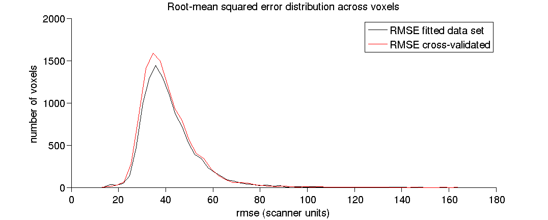
(1.7) Plot a histogram of the RMSE.

We plot the histogram of RMSE across white-mater voxels.

[fh(1), ~, ~] = plotHistRMSE(prob);

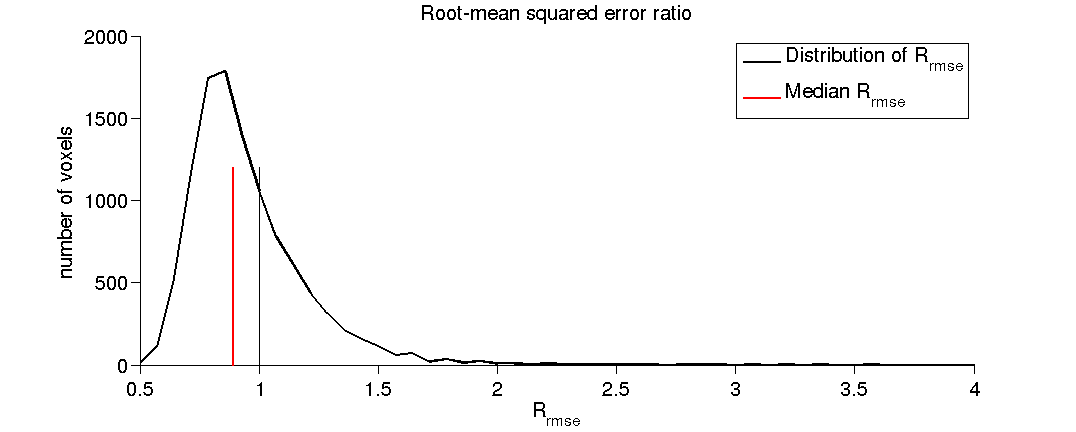
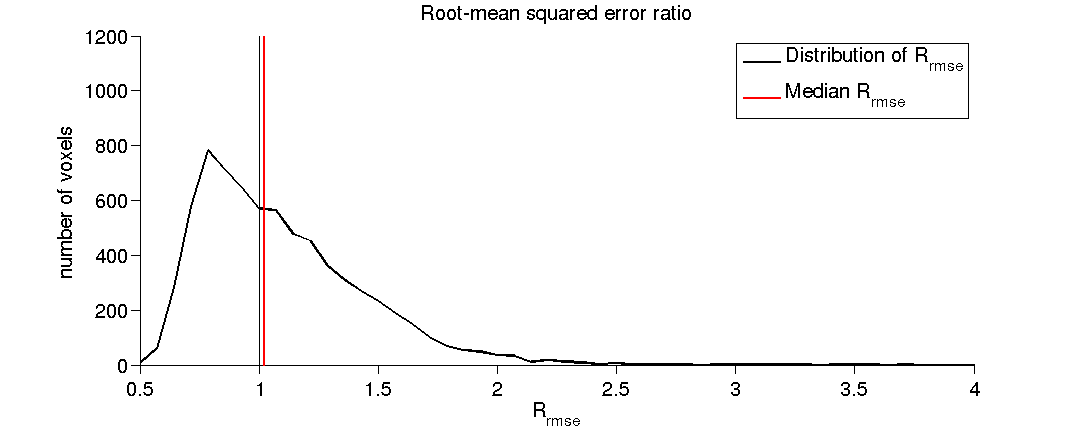
(1.8) Plot a histogram of the RMSE ratio.

As a reminder the Rrmse is the ratio between data test-retest reliability and model error (the quality of the model fit).

[fh(2), ~] = plotHistRrmse(prob);

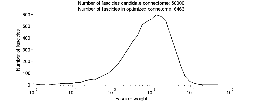
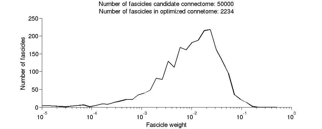
(1.9) Plot a histogram of the fitted fascicle weights.

[fh(3), ~] = plotHistWeigths(prob);
fe = feConnectomeInit(dwiFile,fgFileName,feFileName,[],dwiFileRepeat,t1File);

[feOpenLocalCluster] Found Matlab parallel cluster open, not intializing.

[feConnectomeInit]
 loading fiber from file: /marcovaldo/frk/git/life/Pestilli_etal_manuscript/data/tractography/pestilli_et_al_life_demo_mrtrix_csd_lmax10_probabilistic.mat

[feConnectomeInit] Computing fibers' tensors... [feOpenLocalCluster] Found Matlab parallel cluster open, not intializing.
Elapsed time is 3.185436 seconds.
[fefgGet] Computing fibers/nodes pairing in each voxel..
[fefgGet] Computing nodes-to-voxels..[feOpenLocalCluster] Found Matlab parallel cluster open, not intializing.
 took: 0.494minutes.
[fefgGet] Computing voxels-in-fg..[feOpenLocalCluster] Found Matlab parallel cluster open, not intializing.
 took: 0.243s.
[fefgGet] Computing nodes-in-voxels..[feOpenLocalCluster] Found Matlab parallel cluster open, not intializing.
 took: 0.208s.
[fefgGet] fiber/node pairing completed in: 14.625s.

Files loaded: 
  dwi   = /marcovaldo/frk/git/life/Pestilli_etal_manuscript/data/diffusion/pestilli_etal_life_demo_scan1_subject1_b2000_150dirs_stanford.nii.gz 
  bvecs = /marcovaldo/frk/git/life/Pestilli_etal_manuscript/data/diffusion/pestilli_etal_life_demo_scan1_subject1_b2000_150dirs_stanford.bvecs 
  bvals = /marcovaldo/frk/git/life/Pestilli_etal_manuscript/data/diffusion/pestilli_etal_life_demo_scan1_subject1_b2000_150dirs_stanford.bvals


Files loaded: 
  dwi   = /marcovaldo/frk/git/life/Pestilli_etal_manuscript/data/diffusion/pestilli_etal_life_demo_scan2_subject1_b2000_150dirs_stanford.nii.gz 
  bvecs = /marcovaldo/frk/git/life/Pestilli_etal_manuscript/data/diffusion/pestilli_etal_life_demo_scan2_subject1_b2000_150dirs_stanford.bvecs 
  bvals = /marcovaldo/frk/git/life/Pestilli_etal_manuscript/data/diffusion/pestilli_etal_life_demo_scan2_subject1_b2000_150dirs_stanford.bvals

LiFE - Building the connectome model...
LiFE - Predicting diffusion signal in 10694 voxel...
[feOpenLocalCluster] Found Matlab parallel cluster open, not intializing.
LiFE - Prediction computed in: 23.072s.
LiFE - Allocating the model prediction...process completed in 454.717s.
LiFE - DONE Building the connectome model.

Extract the coordinates of the white-matter voxels

We will use this later to compare probabilistic and deterministic models.

p.coords = feGet(fe,'roi coords');
clear fe

(2) Evaluate the Deterministic tensor-based connectome.

We will now analyze the tensor-based Deterministic tractography connectome.

det.tractography = 'Deterministic';
fgFileName    = fullfile(lifeDemoDataPath('tractography'), ...
                'pestilli_et_al_life_demo_mrtrix_tensor_deterministic.mat');

% The final connectome and data astructure will be saved with this name:
feFileName    = 'life_build_model_demo_TENSOR_DET';

(2.1) Initialize the LiFE model structure, 'fe' in the code below.

fe = feConnectomeInit(dwiFile,fgFileName,feFileName,[],dwiFileRepeat,t1File);

[feOpenLocalCluster] Found Matlab parallel cluster open, not intializing.

[feConnectomeInit]
 loading fiber from file: /marcovaldo/frk/git/life/Pestilli_etal_manuscript/data/tractography/pestilli_et_al_life_demo_mrtrix_tensor_deterministic.mat

[feConnectomeInit] Computing fibers' tensors... [feOpenLocalCluster] Found Matlab parallel cluster open, not intializing.
Elapsed time is 3.197990 seconds.
[fefgGet] Computing fibers/nodes pairing in each voxel..
[fefgGet] Computing nodes-to-voxels..[feOpenLocalCluster] Found Matlab parallel cluster open, not intializing.
 took: 0.374minutes.
[fefgGet] Computing voxels-in-fg..[feOpenLocalCluster] Found Matlab parallel cluster open, not intializing.
 took: 0.235s.
[fefgGet] Computing nodes-in-voxels..[feOpenLocalCluster] Found Matlab parallel cluster open, not intializing.
 took: 0.200s.
[fefgGet] fiber/node pairing completed in: 15.727s.

Files loaded: 
  dwi   = /marcovaldo/frk/git/life/Pestilli_etal_manuscript/data/diffusion/pestilli_etal_life_demo_scan1_subject1_b2000_150dirs_stanford.nii.gz 
  bvecs = /marcovaldo/frk/git/life/Pestilli_etal_manuscript/data/diffusion/pestilli_etal_life_demo_scan1_subject1_b2000_150dirs_stanford.bvecs 
  bvals = /marcovaldo/frk/git/life/Pestilli_etal_manuscript/data/diffusion/pestilli_etal_life_demo_scan1_subject1_b2000_150dirs_stanford.bvals


Files loaded: 
  dwi   = /marcovaldo/frk/git/life/Pestilli_etal_manuscript/data/diffusion/pestilli_etal_life_demo_scan2_subject1_b2000_150dirs_stanford.nii.gz 
  bvecs = /marcovaldo/frk/git/life/Pestilli_etal_manuscript/data/diffusion/pestilli_etal_life_demo_scan2_subject1_b2000_150dirs_stanford.bvecs 
  bvals = /marcovaldo/frk/git/life/Pestilli_etal_manuscript/data/diffusion/pestilli_etal_life_demo_scan2_subject1_b2000_150dirs_stanford.bvals

LiFE - Building the connectome model...
LiFE - Predicting diffusion signal in 7078 voxel...
[feOpenLocalCluster] Found Matlab parallel cluster open, not intializing.
LiFE - Prediction computed in: 14.294s.
LiFE - Allocating the model prediction...process completed in 125.694s.
LiFE - DONE Building the connectome model.

(2.2) Fit the model.

Hereafter we fit the forward model of tracrography using a least-squared method. The information generated by fitting the model (fiber weights etc) is then installed in the LiFE structure.

fe = feSet(fe,'fit',feFitModel(feGet(fe,'mfiber'),feGet(fe,'dsigdemeaned'),'bbnnls'));

LiFE: Computing least-square minimization with BBNNLS...
Running: **** SBB-NNLS ****

Iter   	     Obj		  ||pg||_inf		 ||x-x*||
-------------------------------------------------------
0001	 9.970486E+08	5.684343E+07	NaN
0002	 9.679903E+08	2.263819E+07	NaN
0003	 9.512407E+08	1.784371E+07	NaN
0004	 9.338505E+08	1.511434E+07	NaN
0005	 9.297389E+08	1.609285E+07	NaN
0006	 9.258643E+08	1.776848E+07	NaN
0007	 9.235188E+08	1.368366E+07	NaN
0008	 9.210124E+08	9.679174E+06	NaN
0009	 9.105647E+08	9.348851E+06	NaN
0010	 9.144291E+08	8.318802E+06	NaN
0011	 9.011272E+08	4.183678E+07	NaN
0012	 9.005749E+08	7.291729E+06	NaN
0013	 9.000763E+08	7.039439E+06	NaN
0014	 8.968588E+08	7.000123E+06	NaN
0015	 8.959006E+08	8.719003E+06	NaN
0016	 8.954139E+08	6.535597E+06	NaN
0017	 8.951538E+08	6.510339E+06	NaN
0018	 8.943234E+08	6.494179E+06	NaN
0019	 8.936961E+08	6.414160E+06	NaN
0020	 9.182663E+08	6.340702E+06	NaN
0021	 8.848653E+08	6.519158E+07	NaN
0022	 8.838634E+08	5.718379E+06	NaN
0023	 8.829055E+08	4.864422E+06	NaN
0024	 8.821302E+08	4.899005E+06	NaN
0025	 8.816622E+08	4.895295E+06	NaN
0026	 8.811756E+08	4.855169E+06	NaN
0027	 8.806214E+08	5.937712E+06	NaN
0028	 8.804542E+08	4.738092E+06	NaN
0029	 8.802746E+08	4.714609E+06	NaN
0030	 9.153688E+08	4.685794E+06	NaN
0031	 8.783175E+08	3.034392E+07	NaN
0032	 8.763082E+08	1.513730E+07	NaN
0033	 8.757820E+08	7.925455E+06	NaN
0034	 8.745643E+08	6.648885E+06	NaN
0035	 8.739556E+08	5.699390E+06	NaN
0036	 8.727987E+08	5.258446E+06	NaN
0037	 8.716118E+08	1.244945E+07	NaN
0038	 8.714759E+08	3.596560E+06	NaN
0039	 8.713617E+08	3.529087E+06	NaN
0040	 8.700892E+08	3.460989E+06	NaN
0041	 8.701275E+08	6.955399E+06	NaN
0042	 8.698075E+08	8.286403E+06	NaN
0043	 8.697525E+08	4.165024E+06	NaN
0044	 8.696550E+08	2.760522E+06	NaN
0045	 8.695750E+08	4.235092E+06	NaN
0046	 8.695427E+08	2.185471E+06	NaN
0047	 8.695002E+08	2.169553E+06	NaN
0048	 8.694840E+08	2.145955E+06	NaN
0049	 8.687535E+08	9.354907E+06	NaN
0050	 8.687107E+08	1.858194E+06	NaN
0051	 8.686477E+08	1.880950E+06	NaN
0052	 8.682271E+08	1.913882E+06	NaN
0053	 8.681464E+08	2.044168E+06	NaN
0054	 8.681137E+08	1.971895E+06	NaN
0055	 8.680967E+08	1.956302E+06	NaN
0056	 8.678090E+08	1.948326E+06	NaN
0057	 8.677390E+08	1.758367E+06	NaN
0058	 8.677138E+08	1.696132E+06	NaN
0059	 8.676970E+08	1.697779E+06	NaN
0060	 8.672924E+08	1.698081E+06	NaN
0061	 8.663866E+08	1.017256E+07	NaN
0062	 8.662087E+08	3.193056E+06	NaN
0063	 8.661584E+08	1.317881E+06	NaN
0064	 8.660144E+08	1.217811E+06	NaN
0065	 8.659607E+08	1.301806E+06	NaN
0066	 8.658165E+08	1.143631E+06	NaN
0067	 8.657900E+08	1.149969E+06	NaN
0068	 8.656206E+08	1.142268E+06	NaN
0069	 8.655424E+08	1.099635E+06	NaN
0070	 8.654755E+08	1.107508E+06	NaN
0071	 8.653734E+08	4.657662E+06	NaN
0072	 8.653028E+08	4.163549E+06	NaN
0073	 8.652054E+08	3.463419E+06	NaN
0074	 8.651255E+08	2.169527E+06	NaN
0075	 8.651079E+08	1.040916E+06	NaN
0076	 8.651022E+08	1.921179E+06	NaN
0077	 8.650841E+08	2.675824E+06	NaN
0078	 8.650772E+08	1.293092E+06	NaN
0079	 8.650720E+08	1.048236E+06	NaN
0080	 8.650426E+08	9.974732E+05	NaN
0081	 8.650202E+08	2.220582E+06	NaN
0082	 8.650101E+08	9.904039E+05	NaN
0083	 8.649990E+08	9.881975E+05	NaN
0084	 8.647128E+08	9.854661E+05	NaN
0085	 8.640422E+08	1.141021E+07	NaN
0086	 8.640129E+08	2.809706E+06	NaN
0087	 8.640035E+08	1.471573E+06	NaN
0088	 8.640055E+08	1.304384E+06	NaN
0089	 8.639478E+08	2.993906E+06	NaN
0090	 8.639404E+08	7.288329E+05	NaN
0091	 8.639307E+08	6.763584E+05	NaN
0092	 8.638566E+08	6.343543E+05	NaN
0093	 8.638244E+08	1.993708E+06	NaN
0094	 8.638177E+08	1.014115E+06	NaN
0095	 8.638141E+08	6.284270E+05	NaN
0096	 8.637935E+08	6.270324E+05	NaN
0097	 8.637592E+08	1.929580E+06	NaN
0098	 8.637499E+08	5.998237E+05	NaN
0099	 8.637405E+08	6.007184E+05	NaN
0100	 8.632274E+08	6.009706E+05	NaN
0101	 8.631939E+08	1.565404E+06	NaN
0102	 8.631549E+08	2.816085E+06	NaN
0103	 8.631434E+08	1.837533E+06	NaN
0104	 8.631309E+08	1.111112E+06	NaN
0105	 8.631035E+08	2.111516E+06	NaN
0106	 8.630977E+08	6.417667E+05	NaN
0107	 8.630925E+08	5.824417E+05	NaN
0108	 8.631564E+08	5.661267E+05	NaN
0109	 8.630294E+08	3.306234E+06	NaN
0110	 8.630214E+08	6.416115E+05	NaN
0111	 8.630152E+08	4.542014E+05	NaN
0112	 8.629968E+08	4.531067E+05	NaN
0113	 8.629886E+08	4.491968E+05	NaN
0114	 8.629762E+08	4.864040E+05	NaN
0115	 8.629686E+08	1.213038E+06	NaN
0116	 8.629644E+08	4.471330E+05	NaN
0117	 8.629608E+08	4.467213E+05	NaN
0118	 8.627444E+08	4.463453E+05	NaN
0119	 8.627618E+08	1.237948E+06	NaN
0120	 8.627213E+08	2.583731E+06	NaN
0121	 8.627089E+08	1.398782E+06	NaN
0122	 8.627176E+08	1.120255E+06	NaN
0123	 8.626638E+08	2.471098E+06	NaN
0124	 8.626588E+08	5.952156E+05	NaN
0125	 8.626531E+08	4.992019E+05	NaN
0126	 8.626497E+08	4.590894E+05	NaN
0127	 8.626230E+08	1.336456E+06	NaN
0128	 8.626200E+08	4.269363E+05	NaN
0129	 8.626180E+08	3.223169E+05	NaN
0130	 8.626035E+08	3.221922E+05	NaN
0131	 8.625991E+08	4.581946E+05	NaN
0132	 8.625970E+08	3.674037E+05	NaN
0133	 8.625959E+08	2.821452E+05	NaN
0134	 8.625728E+08	3.008199E+05	NaN
0135	 8.625696E+08	3.674944E+05	NaN
0136	 8.625678E+08	4.262321E+05	NaN
0137	 8.625670E+08	3.067988E+05	NaN
0138	 8.626336E+08	3.166774E+05	NaN
0139	 8.625169E+08	3.455281E+06	NaN
0140	 8.625140E+08	6.715164E+05	NaN
0141	 8.625128E+08	3.727452E+05	NaN
0142	 8.625101E+08	2.997351E+05	NaN
0143	 8.625085E+08	4.593136E+05	NaN
0144	 8.625072E+08	2.660445E+05	NaN
0145	 8.625059E+08	2.434259E+05	NaN
0146	 8.624747E+08	2.504516E+05	NaN
0147	 8.624553E+08	1.706518E+06	NaN
0148	 8.624498E+08	5.061963E+05	NaN
0149	 8.624453E+08	3.555962E+05	NaN
0150	 8.624395E+08	2.776407E+05	NaN
0151	 8.624382E+08	2.925206E+05	NaN
0152	 8.624365E+08	2.696830E+05	NaN
0153	 8.624356E+08	3.943150E+05	NaN
0154	 8.624349E+08	2.672684E+05	NaN
0155	 8.624344E+08	2.480222E+05	NaN
0156	 8.624100E+08	2.422513E+05	NaN
0157	 8.623905E+08	2.222566E+06	NaN
0158	 8.623884E+08	8.790332E+05	NaN
0159	 8.623876E+08	4.316724E+05	NaN
0160	 8.623861E+08	3.435185E+05	NaN
0161	 8.623851E+08	5.237838E+05	NaN
0162	 8.623844E+08	1.786993E+05	NaN
0163	 8.623836E+08	1.784642E+05	NaN
0164	 8.623728E+08	1.780562E+05	NaN
0165	 8.623746E+08	7.396972E+05	NaN
0166	 8.623714E+08	1.155687E+06	NaN
0167	 8.623703E+08	6.199973E+05	NaN
0168	 8.623734E+08	4.698479E+05	NaN
0169	 8.623668E+08	1.571705E+06	NaN
0170	 8.623663E+08	3.086571E+05	NaN
0171	 8.623659E+08	2.479452E+05	NaN
0172	 8.623607E+08	2.310118E+05	NaN
0173	 8.623587E+08	7.133116E+05	NaN
0174	 8.623582E+08	2.190418E+05	NaN
0175	 8.623579E+08	1.656421E+05	NaN
0176	 8.623495E+08	1.657471E+05	NaN
0177	 8.623450E+08	1.082842E+06	NaN
0178	 8.623432E+08	7.001350E+05	NaN
0179	 8.623426E+08	4.662767E+05	NaN
0180	 8.623417E+08	3.337069E+05	NaN
0181	 8.623405E+08	6.205345E+05	NaN
0182	 8.623401E+08	2.435010E+05	NaN
0183	 8.623391E+08	2.281339E+05	NaN
0184	 8.623346E+08	1.870134E+05	NaN
0185	 8.623340E+08	3.817217E+05	NaN
0186	 8.623336E+08	2.109631E+05	NaN
0187	 8.623333E+08	1.546169E+05	NaN
0188	 8.623298E+08	1.544063E+05	NaN
0189	 8.623288E+08	4.085241E+05	NaN
0190	 8.623283E+08	2.797397E+05	NaN
0191	 8.623281E+08	2.093119E+05	NaN
0192	 8.623285E+08	1.848978E+05	NaN
0193	 8.623219E+08	1.151813E+06	NaN
0194	 8.623213E+08	2.566446E+05	NaN
0195	 8.623210E+08	1.656123E+05	NaN
0196	 8.623190E+08	1.317044E+05	NaN
0197	 8.623185E+08	2.782998E+05	NaN
0198	 8.623180E+08	2.633923E+05	NaN
0199	 8.623178E+08	2.008870E+05	NaN
0200	 8.623173E+08	1.616648E+05	NaN
0201	 8.623133E+08	7.704667E+05	NaN
0202	 8.623130E+08	1.133142E+05	NaN
0203	 8.623127E+08	1.131689E+05	NaN
0204	 8.623089E+08	1.151124E+05	NaN
0205	 8.623075E+08	1.899335E+05	NaN
0206	 8.623078E+08	1.591956E+05	NaN
0207	 8.623065E+08	4.431207E+05	NaN
0208	 8.623063E+08	1.315774E+05	NaN
0209	 8.623061E+08	1.339833E+05	NaN
0210	 8.622866E+08	1.328851E+05	NaN
0211	 8.622831E+08	4.492929E+05	NaN
0212	 8.622805E+08	2.056172E+05	NaN
0213	 8.622798E+08	1.606012E+05	NaN
0214	 8.622794E+08	1.641043E+05	NaN
0215	 8.622792E+08	2.470579E+05	NaN
0216	 8.622789E+08	1.120607E+05	NaN
0217	 8.622786E+08	1.120190E+05	NaN
0218	 8.622763E+08	1.119656E+05	NaN
0219	 8.622753E+08	5.556776E+05	NaN
0220	 8.622746E+08	3.955568E+05	NaN
0221	 8.622745E+08	2.505034E+05	NaN
0222	 8.622740E+08	1.189440E+05	NaN
0223	 8.622737E+08	2.805689E+05	NaN
0224	 8.622736E+08	1.119510E+05	NaN
0225	 8.622735E+08	1.119375E+05	NaN
0226	 8.622668E+08	1.119252E+05	NaN
0227	 8.622660E+08	2.308600E+05	NaN
0228	 8.622654E+08	2.630017E+05	NaN
0229	 8.622652E+08	2.639938E+05	NaN
0230	 8.622649E+08	1.106993E+05	NaN
0231	 8.622647E+08	1.106250E+05	NaN
0232	 8.622635E+08	1.105682E+05	NaN
0233	 8.622633E+08	1.630468E+05	NaN
0234	 8.622631E+08	2.125581E+05	NaN
0235	 8.622630E+08	1.242981E+05	NaN
0236	 8.622627E+08	8.041950E+04	NaN
0237	 8.622626E+08	7.541519E+04	NaN
0238	 8.622625E+08	7.591745E+04	NaN
0239	 8.622620E+08	2.255220E+05	NaN
0240	 8.622619E+08	7.383824E+04	NaN
0241	 8.622619E+08	7.316794E+04	NaN
0242	 8.622524E+08	7.283062E+04	NaN
0243	 8.622514E+08	3.926528E+05	NaN
0244	 8.622501E+08	3.153857E+05	NaN
0245	 8.622496E+08	2.112597E+05	NaN
0246	 8.622493E+08	1.590563E+05	NaN
0247	 8.622490E+08	1.586902E+05	NaN
0248	 8.622489E+08	1.437092E+05	NaN
0249	 8.622488E+08	1.415864E+05	NaN
0250	 8.622484E+08	1.386262E+05	NaN
0251	 8.622483E+08	1.167328E+05	NaN
0252	 8.622482E+08	1.135212E+05	NaN
0253	 8.622482E+08	1.106881E+05	NaN
0254	 8.622481E+08	1.092259E+05	NaN
0255	 8.622479E+08	1.063344E+05	NaN
0256	 8.622500E+08	9.847775E+04	NaN
0257	 8.622477E+08	8.056700E+05	NaN
0258	 8.622466E+08	4.542014E+05	NaN
0259	 8.622461E+08	2.532999E+05	NaN
0260	 8.622456E+08	1.980741E+05	NaN
0261	 8.622455E+08	2.021017E+05	NaN
0262	 8.622454E+08	1.128524E+05	NaN
0263	 8.622451E+08	2.520059E+05	NaN
0264	 8.622451E+08	7.682183E+04	NaN
0265	 8.622450E+08	7.568261E+04	NaN
0266	 8.622443E+08	7.430076E+04	NaN
0267	 8.622444E+08	7.415195E+04	NaN
0268	 8.622442E+08	2.121541E+05	NaN
0269	 8.622440E+08	2.605170E+05	NaN
0270	 8.622440E+08	5.949187E+04	NaN
0271	 8.622440E+08	4.577448E+04	NaN
0272	 8.622438E+08	4.522509E+04	NaN
0273	 8.622438E+08	4.434584E+04	NaN
0274	 8.622439E+08	4.483865E+04	NaN
0275	 8.622436E+08	2.416356E+05	NaN
0276	 8.622436E+08	1.411188E+05	NaN
0277	 8.622435E+08	7.159837E+04	NaN
0278	 8.622435E+08	4.654989E+04	NaN
0279	 8.622435E+08	4.454437E+04	NaN
0280	 8.622434E+08	4.447708E+04	NaN
0281	 8.622434E+08	4.439837E+04	NaN
0282	 8.622433E+08	4.440887E+04	NaN
0283	 8.622433E+08	4.439797E+04	NaN
0284	 8.622432E+08	4.440607E+04	NaN
0285	 8.622432E+08	4.430821E+04	NaN
0286	 8.622431E+08	4.436997E+04	NaN
0287	 8.622431E+08	4.438358E+04	NaN
0288	 8.622416E+08	4.438594E+04	NaN
0289	 8.622460E+08	3.506194E+05	NaN
0290	 8.622430E+08	1.001494E+06	NaN
0291	 8.622422E+08	5.477185E+05	NaN
0292	 8.622427E+08	3.839422E+05	NaN
0293	 8.622403E+08	8.008142E+05	NaN
0294	 8.622402E+08	2.124078E+05	NaN
0295	 8.622401E+08	1.388111E+05	NaN
0296	 8.622399E+08	1.131968E+05	NaN
0297	 8.622399E+08	1.188683E+05	NaN
0298	 8.622399E+08	5.015879E+04	NaN
0299	 8.622399E+08	4.626881E+04	NaN
0300	 8.622398E+08	4.558621E+04	NaN
0301	 8.622398E+08	4.538590E+04	NaN
0302	 8.622413E+08	4.513148E+04	NaN
0303	 8.622396E+08	4.315968E+05	NaN
0304	 8.622395E+08	4.394712E+04	NaN
0305	 8.622395E+08	4.385522E+04	NaN
0306	 8.622394E+08	4.382889E+04	NaN
0307	 8.622394E+08	4.378768E+04	NaN
0308	 8.622395E+08	4.361678E+04	NaN
0309	 8.622393E+08	1.300064E+05	NaN
0310	 8.622393E+08	9.054178E+04	NaN
0311	 8.622393E+08	4.375161E+04	NaN
0312	 8.622392E+08	4.357385E+04	NaN
0313	 8.622392E+08	4.310026E+04	NaN
0314	 8.622392E+08	4.332259E+04	NaN
0315	 8.622392E+08	4.351549E+04	NaN
0316	 8.622391E+08	4.339588E+04	NaN
0317	 8.622391E+08	4.344295E+04	NaN
0318	 8.622391E+08	4.330778E+04	NaN
0319	 8.622391E+08	4.337200E+04	NaN
0320	 8.622391E+08	4.333007E+04	NaN
0321	 8.622391E+08	4.330965E+04	NaN
0322	 8.622757E+08	4.331629E+04	NaN
0323	 8.622656E+08	1.887147E+06	NaN
0324	 8.622606E+08	9.945697E+05	NaN
0325	 8.622575E+08	8.207699E+05	NaN
0326	 8.622515E+08	8.116771E+05	NaN
0327	 8.622492E+08	8.235845E+05	NaN
0328	 8.622471E+08	7.548131E+05	NaN
0329	 8.622460E+08	7.234865E+05	NaN
0330	 8.622491E+08	7.005923E+05	NaN
0331	 8.622402E+08	1.269059E+06	NaN
0332	 8.622398E+08	3.803227E+05	NaN
0333	 8.622395E+08	3.679037E+05	NaN
0334	 8.622389E+08	3.537022E+05	NaN
0335	 8.622387E+08	3.154509E+05	NaN
0336	 8.622386E+08	2.950857E+05	NaN
0337	 8.622384E+08	2.693104E+05	NaN
0338	 8.622383E+08	2.625499E+05	NaN
0339	 8.622382E+08	2.564084E+05	NaN
0340	 8.622374E+08	2.489736E+05	NaN
0341	 8.622387E+08	8.701026E+04	NaN
0342	 8.622377E+08	4.641238E+05	NaN
0343	 8.622375E+08	3.768684E+05	NaN
0344	 8.622374E+08	1.446130E+05	NaN
0345	 8.622372E+08	2.232311E+05	NaN
0346	 8.622372E+08	6.394690E+04	NaN
0347	 8.622372E+08	6.397207E+04	NaN
0348	 8.622372E+08	6.395904E+04	NaN
0349	 8.622370E+08	1.732400E+05	NaN
0350	 8.622370E+08	5.943366E+04	NaN
0351	 8.622370E+08	5.862069E+04	NaN
0352	 8.622370E+08	5.766240E+04	NaN
0353	 8.622370E+08	5.366311E+04	NaN
0354	 8.622370E+08	5.128419E+04	NaN
0355	 8.622369E+08	1.002425E+05	NaN
0356	 8.622369E+08	4.205152E+04	NaN
0357	 8.622369E+08	4.169169E+04	NaN
0358	 8.622369E+08	4.123430E+04	NaN
0359	 8.622369E+08	2.596072E+04	NaN
0360	 8.622368E+08	4.531333E+04	NaN
0361	 8.622368E+08	4.572842E+04	NaN
0362	 8.622368E+08	2.317339E+04	NaN
0363	 8.622368E+08	2.298289E+04	NaN
0364	 8.622368E+08	2.276306E+04	NaN
0365	 8.622368E+08	1.776464E+04	NaN
0366	 8.622369E+08	1.864290E+04	NaN
0367	 8.622368E+08	9.408717E+04	NaN
0368	 8.622368E+08	2.849485E+04	NaN
0369	 8.622368E+08	1.499133E+04	NaN
0370	 8.622368E+08	1.499205E+04	NaN
0371	 8.622368E+08	1.499501E+04	NaN
0372	 8.622368E+08	1.499634E+04	NaN
0373	 8.622368E+08	1.901574E+04	NaN
0374	 8.622368E+08	1.500325E+04	NaN
0375	 8.622368E+08	1.500391E+04	NaN
0376	 8.622365E+08	1.500458E+04	NaN
0377	 8.622366E+08	3.780868E+04	NaN
0378	 8.622365E+08	8.841403E+04	NaN
0379	 8.622365E+08	1.495889E+05	NaN
0380	 8.622365E+08	2.104809E+04	NaN
0381	 8.622365E+08	2.078947E+04	NaN
0382	 8.622365E+08	2.037119E+04	NaN
0383	 8.622365E+08	1.554696E+04	NaN
0384	 8.622365E+08	2.510969E+04	NaN
0385	 8.622365E+08	5.004922E+04	NaN
0386	 8.622365E+08	3.977053E+04	NaN
0387	 8.622365E+08	1.513050E+04	NaN
0388	 8.622365E+08	1.512707E+04	NaN
0389	 8.622365E+08	1.510562E+04	NaN
0390	 8.622365E+08	1.510004E+04	NaN
0391	 8.622365E+08	1.508271E+04	NaN
0392	 8.622365E+08	1.508035E+04	NaN
0393	 8.622365E+08	1.507743E+04	NaN
0394	 8.622364E+08	1.507522E+04	NaN
0395	 8.622365E+08	2.651359E+04	NaN
0396	 8.622364E+08	1.649344E+05	NaN
0397	 8.622363E+08	1.955891E+05	NaN
0398	 8.622363E+08	4.219090E+04	NaN
0399	 8.622363E+08	1.539031E+04	NaN
0400	 8.622363E+08	1.488803E+04	NaN
0401	 8.622363E+08	1.494106E+04	NaN
0402	 8.622363E+08	1.768123E+04	NaN
0403	 8.622363E+08	1.494231E+04	NaN
0404	 8.622363E+08	1.494265E+04	NaN
0405	 8.622363E+08	1.494325E+04	NaN
0406	 8.622363E+08	1.494545E+04	NaN
0407	 8.622362E+08	1.850085E+05	NaN
0408	 8.622362E+08	1.133771E+05	NaN
0409	 8.622362E+08	8.030507E+04	NaN
0410	 8.622362E+08	6.646585E+04	NaN
0411	 8.622361E+08	4.455945E+04	NaN
0412	 8.622361E+08	3.330116E+04	NaN
0413	 8.622361E+08	5.668698E+04	NaN
0414	 8.622361E+08	1.966786E+04	NaN
0415	 8.622361E+08	1.877733E+04	NaN
0416	 8.622361E+08	1.730647E+04	NaN
0417	 8.622361E+08	1.525335E+04	NaN
0418	 8.622361E+08	6.920025E+04	NaN
0419	 8.622361E+08	6.512195E+04	NaN
0420	 8.622361E+08	3.563328E+04	NaN
0421	 8.622361E+08	1.553510E+04	NaN
0422	 8.622361E+08	1.517431E+04	NaN
0423	 8.622361E+08	1.507014E+04	NaN
0424	 8.622361E+08	1.507341E+04	NaN
0425	 8.622361E+08	1.507423E+04	NaN
0426	 8.622361E+08	1.507448E+04	NaN
0427	 8.622361E+08	1.507465E+04	NaN
0428	 8.622360E+08	1.507462E+04	NaN
0429	 8.622360E+08	1.506305E+04	NaN
0430	 8.622360E+08	4.552230E+04	NaN
0431	 8.622360E+08	1.997001E+04	NaN
0432	 8.622360E+08	1.502127E+04	NaN
0433	 8.622360E+08	1.501765E+04	NaN
0434	 8.622360E+08	1.498877E+04	NaN
0435	 8.622360E+08	1.486087E+04	NaN
0436	 8.622360E+08	1.489234E+04	NaN
0437	 8.622360E+08	1.491404E+04	NaN
0438	 8.622360E+08	1.492198E+04	NaN
0439	 8.622360E+08	1.493062E+04	NaN
0440	 8.622360E+08	1.493698E+04	NaN
0441	 8.622360E+08	1.509199E+04	NaN
0442	 8.622360E+08	3.457549E+04	NaN
0443	 8.622360E+08	4.065521E+04	NaN
0444	 8.622360E+08	1.631767E+04	NaN
0445	 8.622360E+08	1.502829E+04	NaN
0446	 8.622359E+08	1.502490E+04	NaN
0447	 8.622360E+08	2.948754E+04	NaN
0448	 8.622379E+08	1.148867E+05	NaN
0449	 8.622367E+08	5.830855E+05	NaN
0450	 8.622362E+08	3.154344E+05	NaN
0451	 8.622360E+08	1.798689E+05	NaN
0452	 8.622359E+08	1.514144E+05	NaN
0453	 8.622359E+08	1.329105E+05	NaN
0454	 8.622359E+08	7.616903E+04	NaN
0455	 8.622359E+08	9.693814E+04	NaN
0456	 8.622359E+08	1.225341E+04	NaN
0457	 8.622359E+08	1.448827E+04	NaN
0458	 8.622359E+08	1.104904E+04	NaN
0459	 8.622359E+08	1.422550E+04	NaN
0460	 8.622359E+08	9.311210E+03	NaN
0461	 8.622359E+08	9.314992E+03	NaN
0462	 8.622359E+08	9.317169E+03	NaN
0463	 8.622359E+08	9.321176E+03	NaN
0464	 8.622359E+08	9.324126E+03	NaN
0465	 8.622358E+08	7.003046E+04	NaN
0466	 8.622358E+08	9.286638E+03	NaN
0467	 8.622358E+08	9.266726E+03	NaN
0468	 8.622358E+08	9.244935E+03	NaN
0469	 8.622358E+08	8.943003E+03	NaN
0470	 8.622358E+08	8.923271E+03	NaN
0471	 8.622358E+08	1.372639E+04	NaN
0472	 8.622358E+08	8.873010E+03	NaN
0473	 8.622358E+08	8.867697E+03	NaN
0474	 8.622358E+08	8.863601E+03	NaN
0475	 8.622358E+08	8.803133E+03	NaN
0476	 8.622358E+08	8.791243E+03	NaN
0477	 8.622358E+08	2.925152E+04	NaN
0478	 8.622358E+08	8.747003E+03	NaN
0479	 8.622358E+08	8.744212E+03	NaN
0480	 8.622358E+08	8.740182E+03	NaN
0481	 8.622358E+08	8.649266E+03	NaN
0482	 8.622358E+08	8.644108E+03	NaN
0483	 8.622358E+08	8.634486E+03	NaN
0484	 8.622358E+08	8.632029E+03	NaN
0485	 8.622358E+08	8.628084E+03	NaN
0486	 8.622358E+08	8.626011E+03	NaN
0487	 8.622358E+08	8.596074E+03	NaN
0488	 8.622358E+08	8.593641E+03	NaN
0489	 8.622358E+08	8.571916E+03	NaN
0490	 8.622358E+08	8.570185E+03	NaN
0491	 8.622358E+08	8.567259E+03	NaN
0492	 8.622356E+08	8.564584E+03	NaN
0493	 8.622378E+08	1.316558E+05	NaN
0494	 8.622362E+08	6.380990E+05	NaN
0495	 8.622359E+08	4.855094E+05	NaN
0496	 8.622364E+08	1.883682E+05	NaN
0497	 8.622355E+08	4.741436E+05	NaN
0498	 8.622355E+08	7.989413E+04	NaN
0499	 8.622355E+08	6.274112E+04	NaN
BBNNLS status: Success
Reason: Maximum number of iterations reached
 ...fit process completed in 4.985minutes

(2.3) Extract the RMSE of the model on the fitted data set.

We now use the LiFE structure and the fit to compute the error in each white-matter voxel spanned by the tractography model.

det.rmse   = feGet(fe,'vox rmse');

(2.4) Extract the RMSE of the model on the second data set.

Here we show how to compute the cross-valdiated RMSE of the tractography model in each white-matter voxel. We store this information for later use and to save computer memory.

det.rmsexv = feGetRep(fe,'vox rmse');

(2.5) Extract the Rrmse.

We show how to extract the ratio between the model prediction error (RMSE) and the test-retest reliability of the data.

det.rrmse  = feGetRep(fe,'vox rmse ratio');

(2.6) Extract the fitted weights for the fascicles.

The following line shows how to extract the weight assigned to each fascicle in the connectome.

det.w      = feGet(fe,'fiber weights');

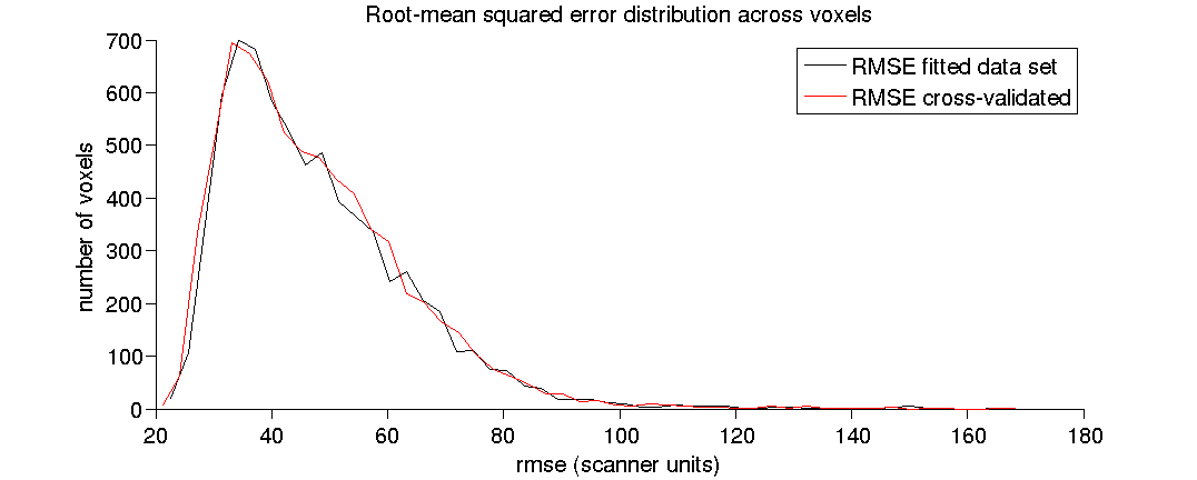
(2.7) Plot a histogram of the RMSE.

We plot the histogram of RMSE across white-mater voxels.

[fh(1), ~, ~] = plotHistRMSE(det);

(2.8) Plot a histogram of the RMSE ratio.

As a reminder the Rrmse is the ratio between data test-retest reliability and model error (the quality of the model fit).

[fh(2), ~] = plotHistRrmse(det);

(2.9) Plot a histogram of the fitted fascicle weights.

[fh(3), ~] = plotHistWeigths(det);

Extract the coordinates of the white-matter voxels.

We will use this later to compare probabilistic and deterministic models.

d.coords = feGet( fe, 'roi coords');
clear fe

(3) Compare the quality of fit of Probabilistic and Deterministic connectomes.

(3.1) Find the common coordinates between the two connectomes.

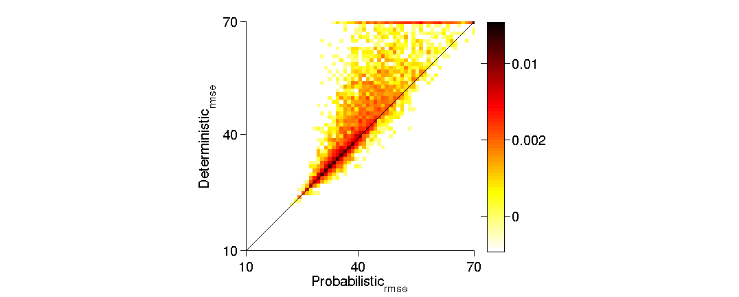
The two tractography method might have passed through slightly different white-matter voxels. Here we find the voxels where both models passed. We will compare the error only in these common voxels. There are more coordinates in the Prob connectome, because the tracking fills up more White-matter.

So, hereafter: - First we find the indices in the probabilistic connectome of the coordinate in the deterministic connectome. But there are some of the coordinates in the Deterministic conectome that are NOT in the Probabilistic connectome.

- Second we find the indices in the Deterministic connectome of the subset of coordinates in the Probabilistic connectome found in the previous step.

- Third we find the common voxels. These allow us to find the rmse for the same voxels.

fprintf('Finding common brain coordinates between P and D connectomes...\n')
prob.coordsIdx = ismember(p.coords,d.coords,'rows');
prob.coords    = p.coords(prob.coordsIdx,:);
det.coordsIdx  = ismember(d.coords,prob.coords,'rows');
det.coords     = d.coords(det.coordsIdx,:);
prob.rmse      = prob.rmse( prob.coordsIdx);
det.rmse       = det.rmse( det.coordsIdx);
clear p d

Finding common brain coordinates between P and D connectomes...

(3.2) Make a scatter plot of the RMSE of the two tractography models

fh(4) = scatterPlotRMSE(det,prob);

(3.3) Compute the strength-of-evidence (S) and the Earth Movers Distance.

Compare the RMSE of the two models using the Stregth-of-evidence and the Earth Movers Distance.

se = feComputeEvidence(prob.rmse,det.rmse);

[feComputeEvidence] Computing the Earth Mover's distance... 
[feComputeEvidence] Computing the Strength of Evidence... 
..... done.

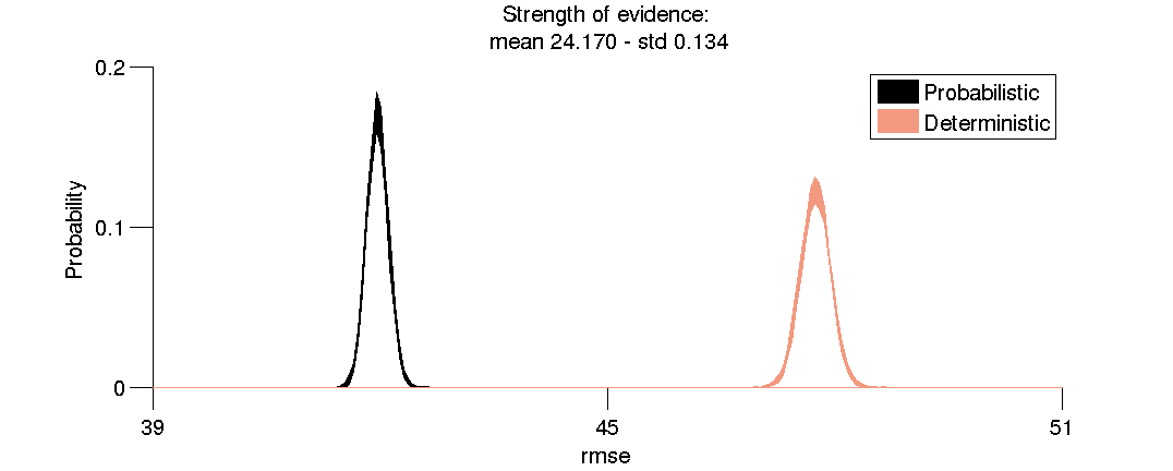
(3.4) Strength of evidence in favor of Probabilistic tractography.

Plot the distributions of resampled mean RMSE used to compute the strength of evidence (S).

fh(5) = distributionPlotStrengthOfEvidence(se);

(3.5) RMSE distributions for Probabilistic and Deterministic tractography.

Compare the distributions using the Earth Movers Distance. Plot the distributions of RMSE for the two models and report the Earth Movers Distance between the distributions.

fh(6) = distributionPlotEarthMoversDistance(se);

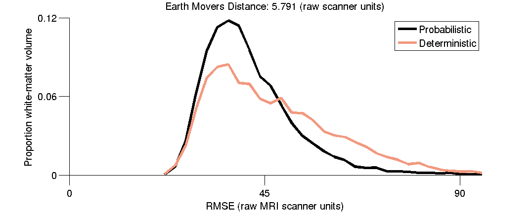
end

% ---------- Local Plot Functions ----------- %
function [fh, rmse, rmsexv] = plotHistRMSE(info)
% Make a plot of the RMSE:
rmse   = info.rmse;
rmsexv = info.rmsexv;

figName = sprintf('%s - RMSE',info.tractography);
fh = mrvNewGraphWin(figName);
[y,x] = hist(rmse,50);
plot(x,y,'k-');
hold on
[y,x] = hist(rmsexv,50);
plot(x,y,'r-');
set(gca,'tickdir','out','fontsize',16,'box','off');
title('Root-mean squared error distribution across voxels','fontsize',16);
ylabel('number of voxels','fontsize',16);
xlabel('rmse (scanner units)','fontsize',16);
legend({'RMSE fitted data set','RMSE cross-validated'},'fontsize',16);
end

function [fh, R] = plotHistRrmse(info)
% Make a plot of the RMSE Ratio:

R       = info.rrmse;
figName = sprintf('%s - RMSE RATIO',info.tractography);
fh      = mrvNewGraphWin(figName);
[y,x]   = hist(R,linspace(.5,4,50));
plot(x,y,'k-','linewidth',2);
hold on
plot([median(R) median(R)],[0 1200],'r-','linewidth',2);
plot([1 1],[0 1200],'k-');
set(gca,'tickdir','out','fontsize',16,'box','off');
title('Root-mean squared error ratio','fontsize',16);
ylabel('number of voxels','fontsize',16);
xlabel('R_{rmse}','fontsize',16);
legend({sprintf('Distribution of R_{rmse}'),sprintf('Median R_{rmse}')});
end

function [fh, w] = plotHistWeigths(info)
% Make a plot of the weights:

w       = info.w;
figName = sprintf('%s - Distribution of fascicle weights',info.tractography);
fh      = mrvNewGraphWin(figName);
[y,x]   = hist(w( w > 0 ),logspace(-5,-.3,40));
semilogx(x,y,'k-','linewidth',2)
set(gca,'tickdir','out','fontsize',16,'box','off')
title( ...
    sprintf('Number of fascicles candidate connectome: %2.0f\nNumber of fascicles in optimized connetome: %2.0f' ...
    ,length(w),sum(w > 0)),'fontsize',16)
ylabel('Number of fascicles','fontsize',16)
xlabel('Fascicle weight','fontsize',16)
end

function fh = scatterPlotRMSE(det,prob)
figNameRmse = sprintf('prob_vs_det_rmse_common_voxels_map');
fh = mrvNewGraphWin(figNameRmse);
[ymap,x]  = hist3([det.rmse;prob.rmse]',{[10:1:70], [10:1:70]});
ymap = ymap./length(prob.rmse);
sh   = imagesc(flipud(log10(ymap)));
cm   = colormap(flipud(hot)); view(0,90);
axis('square')
set(gca, ...
    'xlim',[1 length(x{1})],...
    'ylim',[1 length(x{1})], ...
    'ytick',[1 (length(x{1})/2) length(x{1})], ...
    'xtick',[1 (length(x{1})/2) length(x{1})], ...
    'yticklabel',[x{1}(end) x{1}(round(end/2)) x{1}(1)], ...
    'xticklabel',[x{1}(1)   x{1}(round(end/2)) x{1}(end)], ...
    'tickdir','out','ticklen',[.025 .05],'box','off', ...
    'fontsize',16,'visible','on')
hold on
plot3([1 length(x{1})],[length(x{1}) 1],[max(ymap(:)) max(ymap(:))],'k-','linewidth',1)
ylabel('Deterministic_{rmse}','fontsize',16)
xlabel('Probabilistic_{rmse}','fontsize',16)
cb = colorbar;
tck = get(cb,'ytick');
set(cb,'yTick',[min(tck)  mean(tck) max(tck)], ...
    'yTickLabel',round(1000*10.^[min(tck),...
    mean(tck), ...
    max(tck)])/1000, ...
    'tickdir','out','ticklen',[.025 .05],'box','on', ...
    'fontsize',16,'visible','on')
end

function fh = distributionPlotStrengthOfEvidence(se)

y_e        = se.s.unlesioned_e;
ywo_e      = se.s.lesioned_e;
dprime     = se.s.mean;
std_dprime = se.s.std;
xhis       = se.s.unlesioned.xbins;
woxhis     = se.s.lesioned.xbins;

histcolor{1} = [0 0 0];
histcolor{2} = [.95 .6 .5];
figName = sprintf('Strength_of_Evidence_test_PROB_vs_DET_model_rmse_mean_HIST');
fh = mrvNewGraphWin(figName);
patch([xhis,xhis],y_e(:),histcolor{1},'FaceColor',histcolor{1},'EdgeColor',histcolor{1});
hold on
patch([woxhis,woxhis],ywo_e(:),histcolor{2},'FaceColor',histcolor{2},'EdgeColor',histcolor{2});
set(gca,'tickdir','out', ...
        'box','off', ...
        'ticklen',[.025 .05], ...
        'ylim',[0 .2], ...
        'xlim',[min(xhis) max(woxhis)], ...
        'xtick',[min(xhis) round(mean([xhis, woxhis])) max(woxhis)], ...
        'ytick',[0 .1 .2], ...
        'fontsize',16)
ylabel('Probability','fontsize',16)
xlabel('rmse','fontsize',16')

title(sprintf('Strength of evidence:\n mean %2.3f - std %2.3f',dprime,std_dprime), ...
    'FontSize',16)
legend({'Probabilistic','Deterministic'})
end

function fh = distributionPlotEarthMoversDistance(se)

prob = se.nolesion;
det  = se.lesion;
em   = se.em;

histcolor{1} = [0 0 0];
histcolor{2} = [.95 .6 .5];
figName = sprintf('EMD_PROB_DET_model_rmse_mean_HIST');
fh = mrvNewGraphWin(figName);
plot(prob.xhist,prob.hist,'r-','color',histcolor{1},'linewidth',4);
hold on
plot(det.xhist,det.hist,'r-','color',histcolor{2},'linewidth',4);
set(gca,'tickdir','out', ...
        'box','off', ...
        'ticklen',[.025 .05], ...
        'ylim',[0 .12], ...
        'xlim',[0 95], ...
        'xtick',[0 45 90], ...
        'ytick',[0 .06 .12], ...
        'fontsize',16)
ylabel('Proportion white-matter volume','fontsize',16)
xlabel('RMSE (raw MRI scanner units)','fontsize',16')
title(sprintf('Earth Movers Distance: %2.3f (raw scanner units)',em.mean),'FontSize',16)
legend({'Probabilistic','Deterministic'})
end

ans =

     4     5     6     7     8     9

Contents